Reading sheet music with a neural network.
An optical music recognition model that turns a photograph of a melody into machine-readable ABC notation. A pretrained vision encoder (Google DeepMind's SigLIP-2, partially frozen) feeds a transformer decoder (trained from scratch on ~40,000 tunes, freshly photo-degraded at every pass, using a single consumer GPU).
Photo in, music notation out.
The input is a flat image (phone photo, scan, PDF clipping). The output is structured notation a computer can render, transpose, search, or play back.
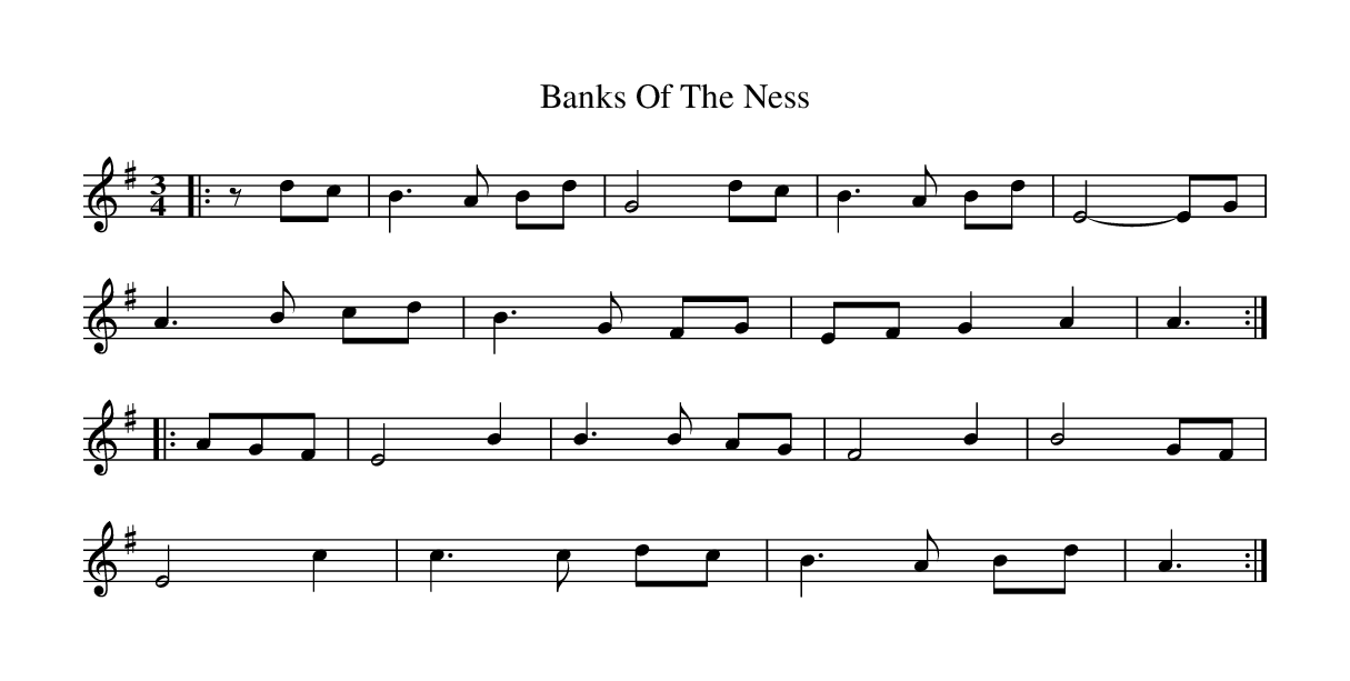
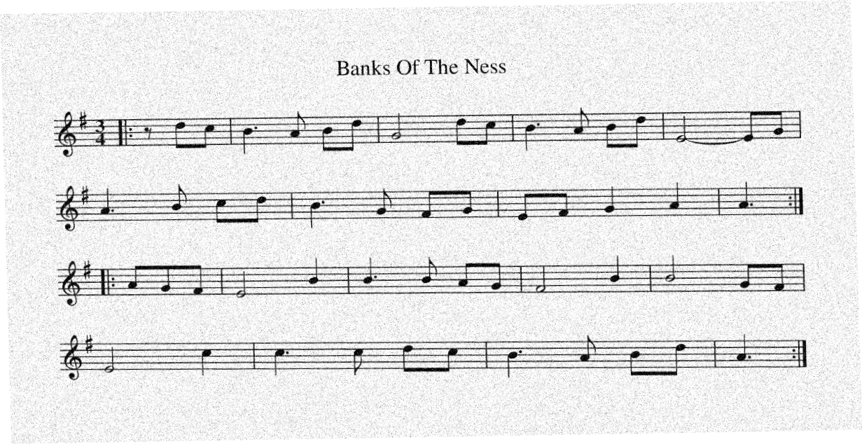 Input
Output
Input
Output
T: Banks Of The Ness
M: 3/4
L: 1/8
K: Gmajor
|:z dc|B3 A Bd|G4 dc|B3 A Bd|E4- EG|A3 B cd|B3 G FG|EF G2 A2|A3:|
|:AGF|E4 B2|B3 B AG|F4 B2|B4 GF|E4 c2|c3 c dc|B3 A Bd|A3:|
A synthetic dataset.
There is no large corpus of photographed sheet music paired with ground
truth ABC scores. Instead, I collected ~50,000 tunes from various archives, engraved each to a pristine PNG with
abcm2ps using several music fonts, then applied physically-motivated augmentations to simulate photographs.
The degradations are sampled fresh each time a tune is drawn, so across a full
training run the model works through roughly a million distinct images without seeing the same photo twice.
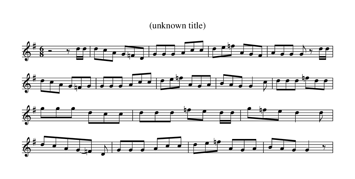 Clean render · source, abcm2ps
Eighteen effects in all: noise, blur, brightness, vignette, rotation, shear, JPEG artifacts, ink bleed, lighting hotspots, resolution loss, and more, were sampled in random combinations.
Encoder-decoder transformers.
The architecture follows the state of the art image-encoder → projector → autoregressive decoder OMR recipe (LEGATO, 2025). A pre-trained large vision model knows how to extract general features from an image. It's kept mostly frozen, but the final four layers are fine-tuned to optimize for musical scores; the rest of the training budget goes into a small decoder that learns to output ABC notation from these features.
SigLIP-2's NaFlex encoder handles variable image dimensions directly, dropping the overlapping-strip segmentation earlier OMR pipelines relied on.
ABC has a ~97-character alphabet, so a 512-token byte-level BPE vocabulary captures common note patterns while keeping the embedding table small and decoding short.
Training details and loss curve.
The objective is token-level cross-entropy, the next-token negative log-likelihood that is standard for autoregressive decoders.
Training used AdamW, a cosine rate schedule with warmup, bf16, and batch size 12, and ran for 96,000 steps — ending during its 29th pass over the training set. The run doesn't stop on loss: every 2,000 steps the model transcribes a fixed set of held-out scores from scratch, and training ends once that transcription accuracy stops improving. The shipped weights are the checkpoint that transcribed best.
Keeping most of the 400M-parameter encoder frozen holds the memory footprint small enough to train the whole model in under a day on a single consumer GPU.
Half of all test images decode with about 2% character error.
Evaluated on 14,970 held-out scores, two-thirds of which carry synthetic photo damage. The headline metric is character error rate (CER): the fraction of characters you'd have to add, delete, or change to turn the prediction into the correct ABC.
The middle of the pack: half of the 14,970 test scores decode with under 2.1% character error. I lead with the median because on a typical score the model is either nearly perfect or perfect; the median reflects the common case, not the tail.
The average over every score. It runs well above the median because a long tail of the longest scores drags it up (the 90th-percentile CER is ~13%), and roughly one score in 130 still diverges outright when the decoder falls into a loop. The gap between mean and median is that tail.
The strictest bar: predictions matching the reference byte-for-byte, headers and all: one in four. No partial credit, so a single stray character fails the whole score.
All numbers use greedy decoding plus one mechanical cleanup: a trailing phrase repeated dozens of times is collapsed to a single copy. The thresholds are conservative, so genuine musical repeats pass through untouched.
A clear path to improvement.
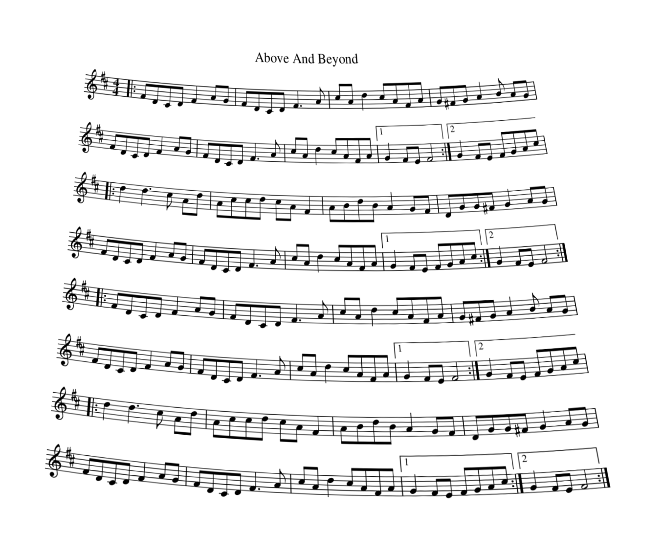
For now, the project has already returned what I wanted from it: a working image-to-ABC pipeline, a clear map of where encoder-decoder OMR strains, and a model that is genuinely usable in practice.
Every training pair is engraved from a handful of music fonts and then photo-degraded. Limited data diversity holds back the model: more engravers, more notation styles, and real captured photographs would allow training beyond what the existing renderer has produced.
CER punishes differences the eye cannot see. For example, extra whitespace or a key labelled "A dorian" instead of "G major" yield the same output. Scoring the rendered notation rather than the raw text would be a better measure of fidelity.
Titles mostly survive now — the current model reads the warped title above correctly — but sung lyrics appear in only 0.2% of training tunes, far too few to learn from, and scores that carry them decode badly. Two options, pulling in opposite directions: mask lyrics out of the loss, or train a second variant that attempts them, and let the user choose.
The worst failures are decode loops: the model repeats a phrase until it hits the token cap. A repetition penalty at decode time made things worse (music legitimately repeats), so the fixes that worked are duller — collapse trailing loops after decoding, and make the early-stopping rule ignore the tail. That cut catastrophic outputs from 2% to under 1% of test scores; ending the remainder likely needs a training objective that penalizes degenerate repetition directly.